Session 17 — Risk–Coverage and Selective Prediction in Medical Imaging UQ 📉
Part 3 — Evaluation of Uncertainty
Forcing a model to answer every question is not always the right design choice. A system that says "I don't know" on uncertain cases — and routes them to a specialist — is often more clinically valuable than one that answers everything with false confidence.
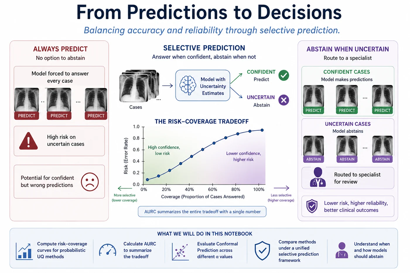
What this notebook covers
- The clinical motivation for selective prediction — why abstention is a feature, not a failure
- Risk and coverage — the two quantities that define the selective prediction tradeoff
- Risk–coverage curves — how error rate changes as the model retains fewer, more confident cases
- AURC — the scalar that summarizes the full risk-coverage tradeoff
- Entropy-based selective prediction for all probabilistic Part 2 methods (VI, MC Dropout, Deep Ensembles, EDL)
- Conformal Prediction evaluated under the same framework — varying $\alpha$ and examining coverage, set efficiency, singleton accuracy
- A conceptual summary of selective prediction as a general framework
🏥 Part 1 — Clinical motivation
Why abstention matters
In most machine learning benchmarks, a model is evaluated on every test example — there is no option to abstain. But in clinical practice, the option to say "I'm not sure — please refer this to a specialist" is not just acceptable; it is often the right answer.
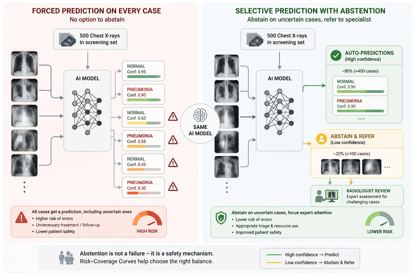
Consider a chest X-ray screening program. The AI model reviews 500 scans per day. For 80% of them, the presentation is clear — obvious consolidation, clean lung fields — and the model's prediction is reliable. For the remaining 20%, the presentation is ambiguous, the image quality is imperfect, or the case falls outside the model's training distribution. Forcing the model to make a definitive prediction on those 20% introduces unnecessary risk.
🎯 Part 2 — The selective prediction framework
A selective classifier answers only when it is confident enough, and defers the rest. The key question is not whether to defer — it is which cases to defer and how many. A good uncertainty estimate makes the model's abstention decisions clinically meaningful: it defers the cases it would likely get wrong, and handles the cases it would get right.
Risk and coverage — the two fundamental quantities
Coverage $c$ is the fraction of cases the model answers (rather than defers):
$$c = \frac{\text{number of cases answered}}{\text{total cases}}$$Risk $R(c)$ is the error rate on the answered cases at coverage level $c$:
$$R(c) = \frac{\text{errors among answered cases}}{\text{answered cases}}$$As coverage decreases (more cases deferred), risk should decrease — because the model retains only the cases it is most confident about. A good uncertainty estimate means the deferred cases are exactly the ones the model would get wrong.
The risk–coverage curve traces $R(c)$ as $c$ varies from 1 (all cases answered) down to 0 (all cases deferred). The shape of this curve tells you how useful the uncertainty estimate is for clinical triage.
📊 Part 3 — AURC: the right scalar for selective prediction
The Area Under the Risk-Coverage Curve (AURC) summarizes the full curve in one number. Lower is better.
$$\text{AURC} = \int_0^1 R(c) \, dc$$where $R(c)$ is the risk at coverage level $c$.
Why AURC and not just accuracy? Accuracy is a single point — 100% coverage. AURC measures the quality of the uncertainty over the full range of coverage levels. A method can have the same accuracy as another but a much better risk-coverage curve — meaning its uncertainty is more useful for clinical triage.
Normalized AURC (NAURC): divides by the random baseline AURC to give a relative score. NAURC=0 means perfect uncertainty (risk drops immediately). NAURC=1 means random uncertainty (no benefit from abstaining).
🔬 Part 4 — Entropy-based selective prediction
For each probabilistic method, we use predictive entropy as the uncertainty score. The selection rule is:
$$\text{answer if } H(x) \leq \tau, \quad \text{defer if } H(x) > \tau$$By sweeping $\tau$ from the minimum to the maximum entropy in the test set, we trace the full risk-coverage curve. We also mark the operating points corresponding to fixed coverage targets (10%, 50%, 90%) that represent realistic clinical deployment scenarios.
Each method is analyzed in its own subsection. No cross-method ranking is made — the goal is to understand each method's selective prediction behaviour independently.
import numpy as np
import pandas as pd
import matplotlib.pyplot as plt
import matplotlib.gridspec as gridspec

from pathlib import Path
from scipy import stats
from statsmodels.stats.proportion import proportions_ztest

np.random.seed(42)

# Load prediction results

RESULTS_DIR = "/kaggle/input/datasets/benyamingheiji/part-2-model-results"

methods_cfg = {
    "VI": ("#7F77DD", f"{RESULTS_DIR}/results_vi.csv"),
    "MC_Dropout": ("#1D9E75", f"{RESULTS_DIR}/results_md.csv"),
    "Deep_Ensembles": ("#E8A838", f"{RESULTS_DIR}/results_de.csv"),
    "EDL": ("#D85A30", f"{RESULTS_DIR}/results_edl.csv"),
}

required_columns = [
    "true_label",
    "mean_pred",
    "pred_label",
]

print("Loading prediction outputs:")

dfs = {}

for method, (_, path) in methods_cfg.items():

    if not Path(path).exists():
        raise FileNotFoundError(
            f"Missing results file for {method}: {path}"
        )

    df = pd.read_csv(path)

    missing = [
        col for col in required_columns
        if col not in df.columns
    ]

    if missing:
        raise ValueError(
            f"{method} is missing required columns: {missing}"
        )

    dfs[method] = df

    print(
        f"  ✅ Loaded {method}: "
        f"{len(df)} samples"
    )

# Load conformal prediction results

cp_path = f"{RESULTS_DIR}/results_cp.csv"

if not Path(cp_path).exists():
    raise FileNotFoundError(
        f"Missing Conformal Prediction results: {cp_path}"
    )

cp_df = pd.read_csv(cp_path)

if (
    "pred_set" in cp_df.columns and
    len(cp_df) > 0 and
    isinstance(cp_df["pred_set"].iloc[0], str)
):
    cp_df["pred_set"] = cp_df["pred_set"].apply(eval)

print(
    f"  ✅ Loaded CP results: "
    f"{len(cp_df)} samples"
)

print("\nReady ✅")
def risk_coverage_curve(correct, uncertainty, n_thresholds=200):
    """
    Sweep uncertainty threshold from low to high.
    At each threshold τ: retain cases with uncertainty ≤ τ.

    Returns:
        coverages  : fraction of cases retained
        risks      : error rate on retained cases
        thresholds : the threshold values swept
    """
    thresholds = np.linspace(uncertainty.min(),
                              uncertainty.max(), n_thresholds)
    coverages, risks = [], []
    for tau in thresholds:
        retained = uncertainty <= tau
        cov = retained.mean()
        risk = 1 - correct[retained].mean() if retained.sum() > 0 else 0.0
        coverages.append(cov)
        risks.append(risk)
    return np.array(coverages), np.array(risks), thresholds


def compute_aurc(coverages, risks):
    """Area Under Risk-Coverage Curve (lower = better)."""
    idx  = np.argsort(coverages)
    return np.trapz(risks[idx], coverages[idx])


def random_baseline_aurc(correct):
    """AURC if uncertainty were random — the baseline to beat."""
    return (1 - correct.mean()) * 0.5


def risk_at_coverage(coverages, risks, target_cov):
    """Risk at a specific coverage target."""
    idx = np.argmin(np.abs(coverages - target_cov))
    return risks[idx]


print('Risk-coverage functions defined ✅')
def analyse_method(name, df, color, coverage_targets=[0.10, 0.50, 0.90]):
    """
    Selective prediction analysis:
    - Risk–coverage curve (formal selective prediction only)
    - No entropy-based grouping or statistical analysis
    """
    correct   = df['correct'].values
    entropy   = df['predictive_entropy'].values
    overall_risk = 1 - correct.mean()

    covs, risks, taus = risk_coverage_curve(correct, entropy)
    aurc      = compute_aurc(covs, risks)
    rand_aurc = random_baseline_aurc(correct)
    naurc     = aurc / rand_aurc if rand_aurc > 0 else 1.0

    fig, ax = plt.subplots(1, 1, figsize=(8, 5))
    fig.suptitle(f'{name} — Selective Prediction Analysis', fontsize=13)


    ax.plot(covs, risks, color=color, linewidth=2.5,
            label=f'Risk-coverage (AURC={aurc:.4f})')

    ax.axhline(overall_risk, color='black', linewidth=1.5,
               linestyle='--', alpha=0.5,
               label=f'Overall risk = {overall_risk:.3f}')

    ax.fill_between(covs, risks, overall_risk,
                    where=(risks < overall_risk),
                    alpha=0.15, color=color)

    op_risks = {}
    for cov_target, marker, ls in zip(
            coverage_targets, ['o','s','D'], ['--','-.',':']):
        r = risk_at_coverage(covs, risks, cov_target)
        op_risks[cov_target] = r

        ax.scatter(cov_target, r, s=100, color=color,
                   marker=marker, zorder=5)

        ax.annotate(f'{cov_target:.0%} cov\n→ {r:.3f} risk',
                    xy=(cov_target, r),
                    xytext=(cov_target - 0.18, r + 0.02),
                    fontsize=8,
                    arrowprops=dict(arrowstyle='->', lw=0.8))

    ax.set_xlabel('Coverage', fontsize=10)
    ax.set_ylabel('Risk (error rate on retained)', fontsize=10)
    ax.set_title('Risk–Coverage curve', fontsize=11)
    ax.legend(fontsize=8)
    ax.spines[['top', 'right']].set_visible(False)

    plt.tight_layout()
    plt.show()

    print(f'\n{name} — Selective Prediction Summary')
    print(f'Overall accuracy : {correct.mean():.4f}')
    print(f'Overall risk     : {overall_risk:.4f}')
    print(f'AURC             : {aurc:.4f}')
    print(f'NAURC            : {naurc:.4f}')

    return {
        'name': name,
        'color': color,
        'covs': covs,
        'risks': risks,
        'aurc': aurc,
        'naurc': naurc,
        'overall_risk': overall_risk,
        'op_risks': op_risks
    }
🔵 4.1 Variational Inference
results_rc = {}
results_rc['VI'] = analyse_method('Variational Inference',
                                  dfs['VI'], '#7F77DD')

🟢 4.2 Monte Carlo Dropout
results_rc['MC_Dropout'] = analyse_method('MC Dropout',
                                           dfs['MC_Dropout'], '#1D9E75')

🟡 4.3 Deep Ensembles
results_rc['Deep_Ensembles'] = analyse_method('Deep Ensembles',
                                               dfs['Deep_Ensembles'], '#E8A838')

🔴 4.4 Evidential Deep Learning
results_rc['EDL'] = analyse_method('Evidential Deep Learning',
                                    dfs['EDL'], '#D85A30')

📊 Part 5 — All risk–coverage curves together
The four curves shown together reveal the shape of each method's risk-coverage tradeoff. No ranking is implied — the curves are shown together for visual reference, not for winner-picking.
fig, axes = plt.subplots(1, 2, figsize=(15, 6))
fig.suptitle('Risk–Coverage curves — all probabilistic methods\n'
             '(each curve reflects a different approach to uncertainty estimation)',
             fontsize=13)

# All curves
for name, res in results_rc.items():
    axes[0].plot(res['covs'], res['risks'],
                 color=res['color'], linewidth=2.0,
                 label=f"{name.replace('_',' ')} (AURC={res['aurc']:.4f})")

# Random baseline
mean_risk = np.mean([r['overall_risk'] for r in results_rc.values()])
axes[0].axhline(mean_risk, color='black', linewidth=1,
                linestyle=':', alpha=0.4,
                label=f'Mean overall risk = {mean_risk:.3f}')

# Operating point lines
for cov, ls in [(0.70,'--'), (0.80,'-.'), (0.90,':')]:
    axes[0].axvline(cov, color='grey', linewidth=1,
                    linestyle=ls, alpha=0.5,
                    label=f'{cov:.0%} coverage target')

axes[0].set_xlabel('Coverage', fontsize=11)
axes[0].set_ylabel('Risk (error rate on retained cases)', fontsize=11)
axes[0].set_title('Risk–Coverage curves', fontsize=12)
axes[0].legend(fontsize=8)
axes[0].spines[['top','right']].set_visible(False)

# AURC bar chart
names  = [n.replace('_',' ') for n in results_rc]
aurcs  = [r['aurc'] for r in results_rc.values()]
colors = [r['color'] for r in results_rc.values()]
bars   = axes[1].bar(names, aurcs, color=colors, alpha=0.75, edgecolor='white')
axes[1].set_ylabel('AURC (lower = better selective prediction)', fontsize=10)
axes[1].set_title('AURC by method', fontsize=12)
axes[1].tick_params(axis='x', rotation=12)
axes[1].spines[['top','right']].set_visible(False)
for bar, v in zip(bars, aurcs):
    axes[1].text(bar.get_x()+bar.get_width()/2,
                 v + 0.0005, f'{v:.4f}',
                 ha='center', fontsize=9)

plt.tight_layout()
plt.show()

# Summary table
print('Selective prediction summary (all methods):')
print(f'{"Method":20s} | {"AURC":>8} | {"NAURC":>8} | '
      f'{"Risk@70%":>10} | {"Risk@80%":>10} | {"Risk@90%":>10}')
print('-' * 88)
for name, res in results_rc.items():
    print(f'{name.replace("_"," "):20s} | {res["aurc"]:8.4f} | '
          f'{res["naurc"]:8.4f} | '
          f'{res["op_risks"][0.10]:10.4f} | '
          f'{res["op_risks"][0.50]:10.4f} | '
          f'{res["op_risks"][0.90]:10.4f} | ')

🎯 Part 6 — Fixed operating points and clinical thresholds
Sweeping the full risk–coverage curve is useful for evaluation, but in real deployment we must choose a single operating point: a decision rule that defines which cases are handled by the AI and which are deferred to a radiologist.
In this work, we focus on two complementary ways of defining such clinical thresholds.
📊 Coverage-based clinical operating points
Coverage-based selection directly controls how many cases the model is allowed to handle. Instead of using a continuous curve, we fix a target retention rate and derive a threshold that enforces it.
We evaluate three clinically meaningful operating points:
90% coverage: the AI handles most cases autonomously, referring only the most uncertain 10%. This prioritizes throughput and scalability.
50% coverage: a balanced setting where the workload is shared equally between AI and radiologist, suitable for decision-support scenarios.
10% coverage: a highly conservative regime where only the most confident predictions are retained, maximizing reliability on handled cases while heavily relying on referral.
These points provide a direct way to translate uncertainty estimates into workload-controlled clinical policies.
🧠 Alternative: data-driven uncertainty thresholds
Beyond predefined coverage levels, another strategy is to derive thresholds directly from the uncertainty distribution.
In our implementation notebooks, we use a clustering-based approach, where predictive uncertainty (e.g., entropy) is grouped into two clusters corresponding to “certain” and “uncertain” predictions. The decision boundary between these clusters is then used as a threshold for clinical triage.
This approach does not require specifying a target coverage in advance. Instead, it allows the data to determine the separation between easy and difficult cases.
🔬 Key interpretation
Both approaches define a single clinical decision boundary, but differ in their philosophy:
Coverage-based thresholding:
“We choose how many cases the AI should handle.”
Clustering-based thresholding:
“We let the data define what is easy vs difficult.”
Together, they represent two complementary strategies for translating uncertainty into clinical decision-making.
coverage_targets = [0.10, 0.50, 0.90]

fig, axes = plt.subplots(1, 3, figsize=(16, 5))
fig.suptitle(
    'Accuracy at fixed clinical coverage levels',
    fontsize=13
)

for ax, cov_target in zip(axes, coverage_targets):

    method_names = [n.replace('_', ' ') for n in results_rc]
    risks_at_cov = [res['op_risks'][cov_target] for res in results_rc.values()]
    colors = [res['color'] for res in results_rc.values()]

    accuracies = [1 - r for r in risks_at_cov]

    bars = ax.bar(
        method_names,
        accuracies,
        color=colors,
        alpha=0.75,
        edgecolor='white'
    )

    overall_accs = [dfs[n]['correct'].mean() for n in results_rc]
    mean_overall = np.mean(overall_accs)

    ax.axhline(
        mean_overall,
        color='black',
        linewidth=1.5,
        linestyle='--',
        alpha=0.5,
        label=f'Overall accuracy = {mean_overall:.3f}'
    )

    ax.set_ylim(0, 1.1)
    ax.set_title(
        f'{cov_target:.0%} coverage\n'
        f'({cov_target:.0%} retained, {1-cov_target:.0%} referred)',
        fontsize=10
    )

    ax.set_ylabel('Accuracy on retained cases')
    ax.tick_params(axis='x', rotation=15, labelsize=8)
    ax.legend(fontsize=8)
    ax.spines[['top', 'right']].set_visible(False)

    for bar, acc in zip(bars, accuracies):
        ax.text(
            bar.get_x() + bar.get_width()/2,
            acc + 0.02,
            f'{acc:.3f}',
            ha='center',
            fontsize=8,
            fontweight='bold'
        )

plt.tight_layout()
plt.show()

ENTROPY_THRESHOLDS = {
    'VI': 0.3612,
    'MC_Dropout': 0.3782,
    'Deep_Ensembles': 0.3920,
    'EDL': 0.3262
}

method_names = [n.replace('_', ' ') for n in results_rc]
colors = [res['color'] for res in results_rc.values()]

cert_accs = []
unc_accs = []

for name in results_rc:

    df = dfs[name]
    entropy = df['predictive_entropy'].values
    correct = df['correct'].values

    thr = ENTROPY_THRESHOLDS[name]

    cert_mask = entropy <= thr
    unc_mask = entropy > thr

    cert_accs.append(correct[cert_mask].mean())
    unc_accs.append(correct[unc_mask].mean())

x = np.arange(len(method_names))
width = 0.35

fig, ax = plt.subplots(1, 1, figsize=(10, 5))

bars1 = ax.bar(x - width/2, cert_accs, width,
               label='Certain (low entropy)',
               color='green', alpha=0.6)

bars2 = ax.bar(x + width/2, unc_accs, width,
               label='Uncertain (high entropy)',
               color='gray', alpha=0.6)

ax.set_xticks(x)
ax.set_xticklabels(method_names, rotation=15)
ax.set_ylim(0, 1.05)

ax.set_ylabel('Accuracy')
ax.set_title('Entropy-based Clustering (Based on Previous Implementation)')
ax.legend()

for bars in [bars1, bars2]:
    for bar in bars:
        ax.text(
            bar.get_x() + bar.get_width()/2,
            bar.get_height() + 0.02,
            f'{bar.get_height():.2f}',
            ha='center',
            fontsize=8
        )

plt.tight_layout()
plt.show()

🟣 Part 7 — Conformal Prediction under the selective prediction framework
Conformal Prediction operates differently from the probabilistic methods. There is no entropy score to threshold. Instead:
- The parameter $\alpha$ controls the target miscoverage rate
- A larger $\alpha$ (e.g. 0.30) → smaller threshold $\hat{\tau}$ → smaller prediction sets → more singletons
- A smaller $\alpha$ (e.g. 0.05) → larger threshold $\hat{\tau}$ → larger prediction sets → fewer singletons
In the selective prediction framework:
- Singleton set ($|C|=1$): the model makes a definitive prediction — analogous to "retained"
- Full set ($|C|=2$): the model cannot distinguish — analogous to "deferred"
We sweep $\alpha$ from 0.01 to 0.10 and track:
- Empirical coverage (does the guarantee hold?)
- Average set size
- Singleton rate (fraction of definitive predictions)
- Accuracy restricted to singleton predictions
# Reconstruct calibration scores from CP results
# We use the nonconf_score column as proxy calibration scores
nc_scores     = cp_df['nonconf_score'].values
test_labels   = cp_df['true_label'].values
test_probs    = cp_df['mean_pred'].values
test_correct  = cp_df['correct'].values

cal_nc_scores = np.load("/kaggle/input/datasets/benyamingheiji/cal-scores/cal_scores.npy")

alpha_values  = np.linspace(0.01, 0.10, 10)
emp_covs, avg_sizes, sing_rates, sing_accs, taus_alpha = [], [], [], [], []

for alpha in alpha_values:
    n_c  = len(cal_nc_scores)
    lvl  = np.ceil((n_c + 1) * (1 - alpha)) / n_c
    tau  = np.quantile(cal_nc_scores, min(lvl, 1.0))
    taus_alpha.append(tau)

    pred_sets, covered_list, sizes = [], [], []
    for i in range(len(test_labels)):
        p   = test_probs[i]
        nc0 = p           # nonconformity for class 0: 1 - p(0) = p(1) = p
        nc1 = 1 - p       # nonconformity for class 1: 1 - p(1) = p(0) = 1-p
        ps  = ([0] if nc0 <= tau else []) + ([1] if nc1 <= tau else [])
        if not ps: ps = [0, 1]
        pred_sets.append(ps)
        covered_list.append(int(test_labels[i] in ps))
        sizes.append(len(ps))

    sizes         = np.array(sizes)
    covered_arr   = np.array(covered_list)
    singleton_mask = sizes == 1

    emp_cov  = covered_arr.mean()
    avg_size = sizes.mean()
    sing_rate = singleton_mask.mean()

    if singleton_mask.sum() > 0:
        # Accuracy on singleton predictions
        singleton_preds  = np.array([
            ps[0] for ps, s in zip(pred_sets, sizes) if s == 1
        ])
        singleton_labels = test_labels[singleton_mask]
        sing_acc = (singleton_preds == singleton_labels).mean()
    else:
        sing_acc = np.nan

    emp_covs.append(emp_cov)
    avg_sizes.append(avg_size)
    sing_rates.append(sing_rate)
    sing_accs.append(sing_acc)

emp_covs   = np.array(emp_covs)
avg_sizes  = np.array(avg_sizes)
sing_rates = np.array(sing_rates)
sing_accs  = np.array(sing_accs)

fig, axes  = plt.subplots(2, 2, figsize=(14, 10))
fig.suptitle('Conformal Prediction — metrics as α varies\n'
             '(larger α = smaller sets, more singletons, lower coverage target)',
             fontsize=13)

# Coverage
axes[0,0].plot(alpha_values, emp_covs, color='#534AB7', linewidth=2.5,
               label='Empirical coverage')
axes[0,0].plot(alpha_values, 1-alpha_values, 'k--', linewidth=1.5,
               alpha=0.5, label='Target (1-α)')
axes[0,0].fill_between(alpha_values, 1-alpha_values, emp_covs,
                        alpha=0.15, color='#1D9E75',
                        label='Coverage slack (guarantee)')
axes[0,0].set_xlabel('α (miscoverage rate)', fontsize=10)
axes[0,0].set_ylabel('Coverage', fontsize=10)
axes[0,0].set_title('Empirical coverage vs target (1-α)\n'
                     'Guarantee: empirical ≥ target always', fontsize=11)
axes[0,0].legend(fontsize=8)
axes[0,0].spines[['top','right']].set_visible(False)

# Average set size
axes[0,1].plot(alpha_values, avg_sizes, color='#7F77DD', linewidth=2.5)
axes[0,1].axhline(1, color='black', linewidth=1, linestyle='--',
                   alpha=0.4, label='Singleton')
axes[0,1].axhline(2, color='black', linewidth=1, linestyle='--',
                   alpha=0.4, label='Full set')
axes[0,1].set_xlabel('α (miscoverage rate)', fontsize=10)
axes[0,1].set_ylabel('Average prediction set size', fontsize=10)
axes[0,1].set_title('Average set size vs α\n'
                     '(larger α → smaller sets)', fontsize=11)
axes[0,1].legend(fontsize=8)
axes[0,1].spines[['top','right']].set_visible(False)

# Singleton rate
axes[1,0].plot(alpha_values, sing_rates, color='#1D9E75', linewidth=2.5,
               label='Singleton rate')
axes[1,0].set_xlabel('α (miscoverage rate)', fontsize=10)
axes[1,0].set_ylabel('Fraction of definitive predictions', fontsize=10)
axes[1,0].set_title('Singleton rate vs α\n'
                     '(larger α → more definitive predictions)',
                     fontsize=11)
axes[1,0].legend(fontsize=9)
axes[1,0].spines[['top','right']].set_visible(False)

# Singleton accuracy
valid = ~np.isnan(sing_accs)
axes[1,1].plot(alpha_values[valid], sing_accs[valid],
               color='#D85A30', linewidth=2.5,
               label='Accuracy on singleton predictions')
overall_acc_cp = cp_df['correct'].mean()
axes[1,1].axhline(overall_acc_cp, color='black', linewidth=1.5,
                   linestyle='--', alpha=0.5,
                   label=f'Overall accuracy = {overall_acc_cp:.3f}')
axes[1,1].set_xlabel('α (miscoverage rate)', fontsize=10)
axes[1,1].set_ylabel('Accuracy', fontsize=10)
axes[1,1].set_title('Accuracy on singleton predictions vs α\n'
                     '(smaller α = more conservative = higher singleton accuracy)',
                     fontsize=11)
axes[1,1].legend(fontsize=8)
axes[1,1].set_ylim(0.5, 1.05)
axes[1,1].spines[['top','right']].set_visible(False)

plt.tight_layout()
plt.show()

# Print table at key alpha values
print('CP metrics at selected α values:')
print(f'{"α":>6} | {"Target cov":>12} | {"Emp. cov":>10} | '
      f'{"Avg size":>10} | {"Singleton %":>12} | {"Singleton acc":>14}')
print('-' * 75)
for a_target in [0, 0.01, 0.03, 0.05, 0.07, 0.09, 0.10]:
    idx = np.argmin(np.abs(alpha_values - a_target))
    print(f'{alpha_values[idx]:6.2f} | {1-alpha_values[idx]:12.2f} | '
          f'{emp_covs[idx]:10.4f} | {avg_sizes[idx]:10.4f} | '
          f'{sing_rates[idx]:11.3f} | '
          f'{sing_accs[idx]:14.4f}' if not np.isnan(sing_accs[idx])
          else f'{alpha_values[idx]:6.2f} | {1-alpha_values[idx]:12.2f} | '
          f'{emp_covs[idx]:10.4f} | {avg_sizes[idx]:10.4f} | '
          f'{sing_rates[idx]:11.3f} |           N/A')

📚 8. Recommended reading
These are the most important papers on risk-coverage, selective prediction, and reject-option learning. They explain where the idea came from, how it works in deep learning, and how modern variants improve the tradeoff between answering and deferring. 🗺️
Selective Classification for Deep Neural Networks
Geifman & El-Yaniv, 2017
A foundational deep-learning paper for selective prediction. It shows how to wrap a trained classifier with a reject option and optimize for a target risk level while controlling coverage.
Bias-Reduced Uncertainty Estimation for Deep Neural Classifiers
Geifman, Uziel & El-Yaniv, 2018
An important follow-up that explains why naive uncertainty scores can be biased and proposes a better estimate for highly confident predictions. Useful for understanding why selective prediction is harder than just thresholding entropy.
SelectiveNet: A Deep Neural Network with an Integrated Reject Option
Geifman & El-Yaniv, 2019
A major modern extension that trains the reject option end-to-end instead of bolting it on after the fact. One of the most cited deep selective classification papers.
A Survey of Selective Classification
Goren, Galil & El-Yaniv, 2024
A recent overview of the field, including hierarchical selective classification and modern evaluation ideas. Good for seeing how the area has evolved beyond the original binary reject setting.
✅ Session summary
| Step | What we did |
|---|---|
| 🏥 Clinical idea | Framed AI as a selective system that can defer uncertain cases to radiologists |
| ⚖️ Core setup | Defined coverage (how many answered) and risk (error on answered set) |
| 📉 Main tool | Built risk–coverage curves to study performance across abstention levels |
| 📏 Key metric | Used AURC / NAURC to summarize uncertainty behavior in one number |
| 🧠 Uncertainty | Used predictive entropy to decide which cases are answered vs deferred |
| 🔵 Methods | Applied VI, MC Dropout, Deep Ensembles, and EDL under the same framework |
| 🚦 Operating points | Evaluated fixed 10%, 50%, 90% coverage clinical settings |
| 📊 Analysis view | Visualized curves and AURC to show selective behavior across methods |
| 🟣 Conformal | Added CP as a set-based method with formal coverage guarantees (α control) |
➡️ Next: Session 18: Out-of-Distribution (OOD) Detection
Session 18 asks what happens when the model meets genuinely unfamiliar data. We move from selective answering to out-of-distribution detection, where the key question is whether the system can recognize when it is outside its validated territory and hand the case off instead of pretending to know.